Comparison
In this section we will compare the fast FFTKDE with three popular implementations.
scipy- scipy.stats.gaussian_kdesklearn- sklearn.neighbors.KernelDensitystatsmodels- statsmodels.nonparametric.kde.KDEUnivariate / statsmodels.nonparametric.kernel_density.KDEMultivariate
This page is inspired by Kernel Density Estimation in Python, where Jake VanderPlas (the original author of the sklearn implementation) compared kernel density estimators in 2013.
Note
Times will vary from computer to computer, and should only be used to compare the relative speed of the algorithms. The CPU used here was an Intel Core i5-6400.
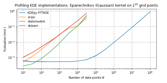
The graph above shows the speed when using an Epanechnikov kernel, for various data sizes.
Feature summary
The table below summarizes the features available across the libraries.
Feature / Library |
scipy |
sklearn |
statsmodels |
KDEpy.FFTKDE |
|---|---|---|---|---|
Number of kernels |
1 (gauss) |
6 |
7 (6 slow) |
9 |
Number of dimensions |
Any |
Any |
Any |
Any |
Weighted data points |
No |
No |
Non-FFT |
Yes |
Automatic bandwidth |
NR |
None |
NR, CV |
NR, ISJ |
Time \(N=10^6\) |
42 s |
22 s |
0.27 s |
0.01 s |
Time \(N=10^2 \times 10^2\) |
0.5 s |
1.6 s |
1.3 s |
0.005 s |
The choice of kernel is typically not important, but it might be nice to experiment with different functions.
Most users will be interested in 1D or 2D estimates, but it’s assuring to know that every implementation generalizes to arbitrary dimensions \(d\).
Being able to weight each data point individually and use a fast algorithm is a great benefit of FFTKDE, which is not found in the other libraries.
statsmodels implements a fast algorithm for unweighed data using the Gaussian kernel in 1D, but everything else runs using a naive algorithm, which is many orders of magnitude slower.
Automatic bandwidth selection is not available out-of-the-box in sklearn, but every other implementation has one or more options.
Normal reference rules (NR) assume a normal distribution when selecting the optimal bandwidth, cross validation (CV) minimizes an error function and the improved Sheather-Jones (ISJ) algorithm provides an asymptotically optimal bandwidth as the number of data points \(N \to \infty\).
The ISJ algorithm is also very robust to multimodal distributions, which NR is not.
The times for the one-dimensional \(N = 10^6\) data points were computed taking the median of 5 runs. The kernel was Gaussian and the number of grid points were chosen to be \(n=2^{10}\). The times for the 2D \(N=10^2 \times 10^2\) data points were also based on the median of 5 runs using a Gaussian kernel.
Speed in 1D
We run the algorithms 20 times on normally distributed data and compare the medians of the running times.
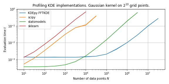
The plot below compares the speed of the implementations with a Gaussian kernel.
The 1D statsmodels implementation uses a similar algorithm when the kernel is Gaussian, and the performance is therefore somewhat comparable.
FFTKDE is initially slower because it solves a non-linear equation to obtain a support threshold for the Gaussian kernel (which does not have finite support).
This is a constant cost, and as \(N \to \infty\) the algorithm is orders of magnitude faster than the competitors.
Switching to the Epanechnikov kernel (scipy falls back to Gaussian, the only kernel implemented) the picture is very different.
FFTKDE knows the support and does not solve an equation, while statsmodels is now forced to use a naive algorithm.
The difference is tremendous.
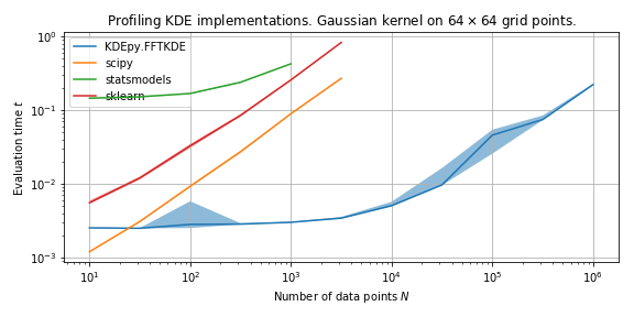
Speed in 2D
We run the 2D algorithms 20 times on normally distributed data and compare medians of the running times.
FFTKDE is fast because of the underlying algorithm – it implements a \(d\)-dimensional linear binning routine and uses \(d\)-dimensional convolution.
Speed as dimension increases
We will now look at how FFTKDE performs as the dimensionality of the data increases.
The plot below shows how speed is affected as the dimension \(d\) increases across different number of data points \(N\).
The running time increases exponentially with \(d\), and this is no surprise as the binning routine has a theoretical runtime \(\mathcal{O}(N 2^d )\).
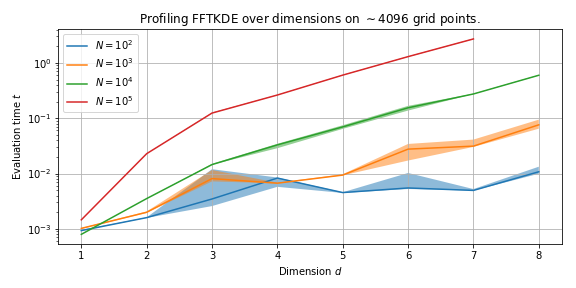
The \(N\)-dimensional binning routine has runtime \(\mathcal{O}(N 2^d)\), and the convolution (using FFT if needed) has runtime \(n \log n\), where \(n\) is the number of grid points. The runtime of the complete algorithm is \(\mathcal{O}\left( N2^d + n \log n\right)\).
