Bandwidth
It is widely accepted in the literature that the choice of bandwidth \(h\) is more important than the choice of kernel \(K\). Consider a kernel density estimator based on \(N\) points, weighting the data points \(x_i\) with weights \(w_i\). We require that \(\sum_i w_i = 1\).
To extend the equation above we divide by a scaling factor \(h\) called the bandwidth. When dividing with \(h\), every dimension \(d\) is stretched, so we must re-scale with \(h^d\) to ensure that \(\int \widehat{f}(x) \, dx\) evaluates to unity.
We will now briefly explain two ways to find a good \(h\).
Note
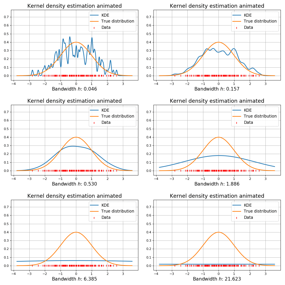
In KDEpy, the bandwidth \(h\) is the standard deviation \(\sigma\) of the kernel function. This is because the implementation contains many kernels, some with finite support and some without, and using \(\sigma\) to quantify the bandwidth allows easy comparison.
The animation below shows kernel density estimation for various choices of \(h\).

Normal reference rules
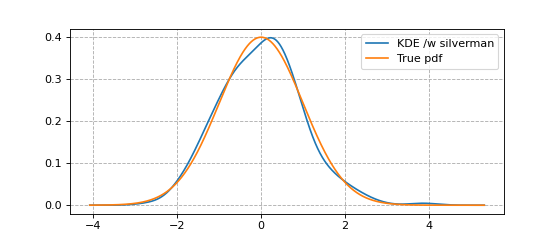
If the data is unimodal and close to normal, silverman’s rule of thumb may be used. It’s computationally very fast, but derived by assuming that the true density is normal. This is somewhat paradoxal, since if we knew that the data was truly normal it would render a kernel density estimator unnecessary.
An example using bw='silverman' is shown in the code snippet below.
from KDEpy import FFTKDE
from scipy.stats import norm

# Generate a distribution and some data
dist = norm(loc=0, scale=1)
data = dist.rvs(2**8) # Generate 2**8 points

# Compute density estimates using 'silverman'
x, y = FFTKDE(kernel='gaussian', bw='silverman').fit(data).evaluate()
plt.plot(x, y, label='KDE /w silverman')

plt.plot(x, dist.pdf(x), label='True pdf')
plt.grid(True, ls='--', zorder=-15); plt.legend();
(Source code, png, hires.png, pdf)

The Improved Sheather-Jones algorithm
If much data is available and the data is far from normal or multimodal, the Improved Sheather Jones (ISJ) algorithm may be used. The Improved Sheather-Jones algorithm is a plug-in selector. The mean integrated square error (MISE) is given by
The ISJ algorithm attempts to find \(h\) to minimize the asymptotic mean integrated square error (AMISE), which depends on the unknown quantity \(\left \| f''(x) \right \|^2\). Using a recursive formula, this is accomplished by computing a sequence of estimates. See the paper by Botev et al in the Literature review for details.
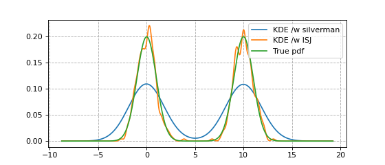
An example using bw='ISJ' is shown in the code snippet below.
With multimodal data, it dramatically outperforms bw='silverman'.
from KDEpy import FFTKDE
from scipy.stats import norm

# Generate a distribution and some multimodal data
dist1 = norm(loc=0, scale=1)
dist2 = norm(loc=10, scale=1)
data = np.hstack([dist1.rvs(2**8), dist2.rvs(2**8)])

# Compute density estimates using 'silverman'
x, y = FFTKDE(kernel='gaussian', bw='silverman').fit(data).evaluate()
plt.plot(x, y, label='KDE /w silverman')

# Compute density estimates using 'ISJ' - Improved Sheather Jones
y = FFTKDE(kernel='gaussian', bw='ISJ').fit(data).evaluate(x)
plt.plot(x, y, label='KDE /w ISJ')

plt.plot(x, (dist1.pdf(x) + dist2.pdf(x))/2, label='True pdf')
plt.grid(True, ls='--', zorder=-15); plt.legend();
(Source code, png, hires.png, pdf)

