Examples

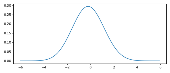
Minimal working example with options

This minimal working example shows how to compute a KDE in one line of code.

from KDEpy import FFTKDE
data = np.random.randn(2**6)

# Notice how bw (standard deviation), kernel, weights and grid points are set
x, y = FFTKDE(bw=1, kernel='gaussian').fit(data, weights=None).evaluate(2**8)

plt.plot(x, y); plt.tight_layout()

(Source code, png, hires.png, pdf)

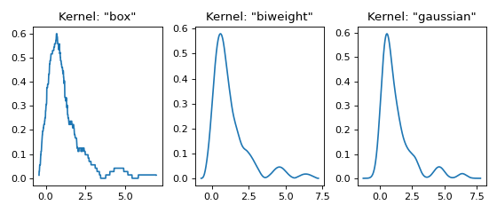
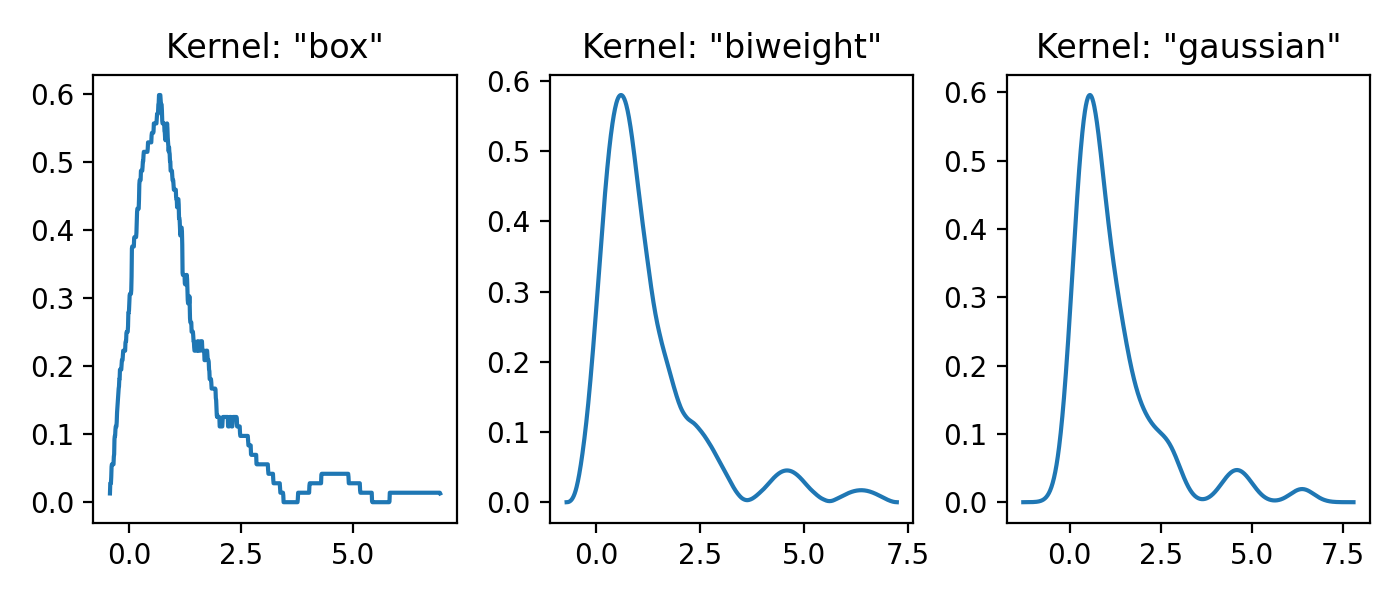
Three kernels in 1D

This example shows the effect of different kernel functions \(K\).

from KDEpy import FFTKDE
data = np.exp(np.random.randn(2**6))  # Lognormal data

for plt_num, kernel in enumerate(['box', 'biweight', 'gaussian'], 1):

    ax = fig.add_subplot(1, 3, plt_num)
    ax.set_title(f'Kernel: "{kernel}"')
    x, y = FFTKDE(kernel=kernel, bw='silverman').fit(data).evaluate()
    ax.plot(x, y)

fig.tight_layout()

(Source code, png, hires.png, pdf)

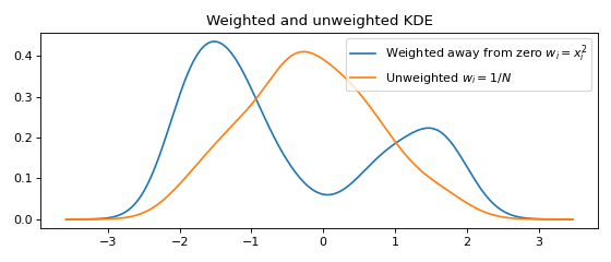
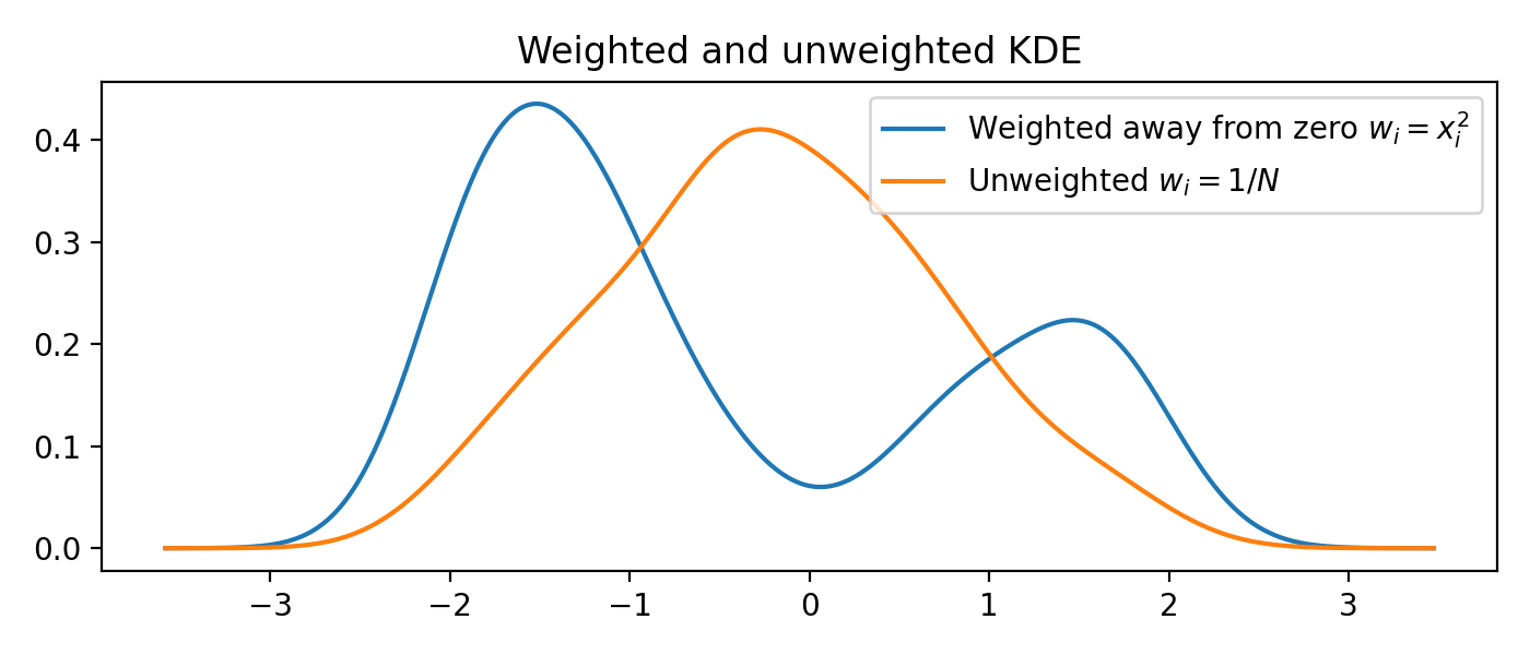
Weighted data

A weight \(w_i\) may be associated with every data point \(x_i\).

from KDEpy import FFTKDE
data = np.random.randn(2**6)  # Normal distribution
weights = data**2  # Large weights away from zero

x, y = FFTKDE(bw='silverman').fit(data, weights).evaluate()
plt.plot(x, y, label=r'Weighted away from zero $w_i = x_i^2$')

y2 = FFTKDE(bw='silverman').fit(data).evaluate(x)
plt.plot(x, y2, label=r'Unweighted $w_i = 1/N$')

plt.title('Weighted and unweighted KDE')
plt.tight_layout(); plt.legend(loc='best');

(Source code, png, hires.png, pdf)

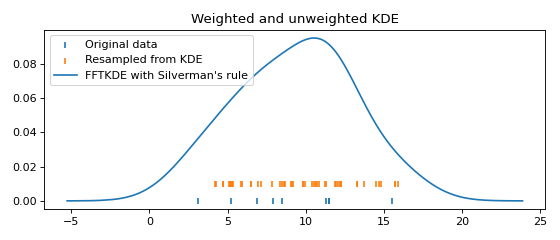
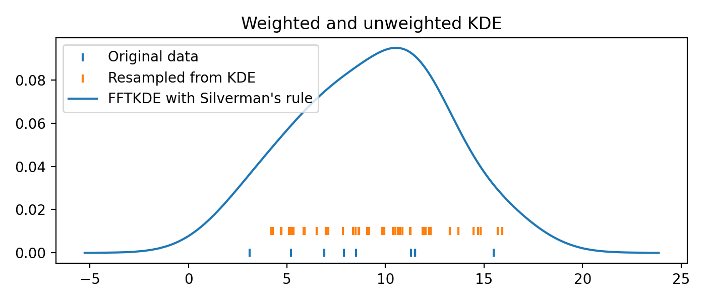
Resampling from the distribution

Resampling data from the fitted KDE is equivalent to (1) first resampling the original data (with replacement), then (2) adding noise drawn from the same probability density as the kernel function in the KDE. Here is an example:

from KDEpy import FFTKDE
from KDEpy.bw_selection import silvermans_rule, improved_sheather_jones

# Get the standard deviation of the kernel functions
data = np.array([3.1, 5.2, 6.9, 7.9, 8.5, 11.3, 11.5, 11.5, 11.5, 15.5])
# Silverman assumes normality of data - use ISJ with much data instead
kernel_std = silvermans_rule(data.reshape(-1, 1))  # Shape (obs, dims)

# (1) First resample original data, then (2) add noise from kernel
size = 50
resampled_data = np.random.choice(data, size=size, replace=True)
resampled_data = resampled_data + np.random.randn(size) * kernel_std

# Plot the results
plt.scatter(data, np.zeros_like(data), marker='|', label="Original data")
plt.scatter(resampled_data, np.ones_like(resampled_data) * 0.01,
            marker='|', label="Resampled from KDE")
x, y = FFTKDE(kernel="gaussian", bw="silverman").fit(data).evaluate()
plt.plot(x, y, label="FFTKDE with Silverman's rule")
plt.title('Weighted and unweighted KDE')
plt.tight_layout(); plt.legend(loc='upper left');

(Source code, png, hires.png, pdf)

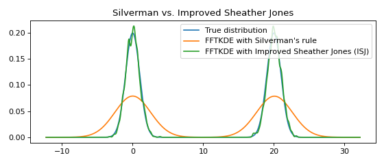
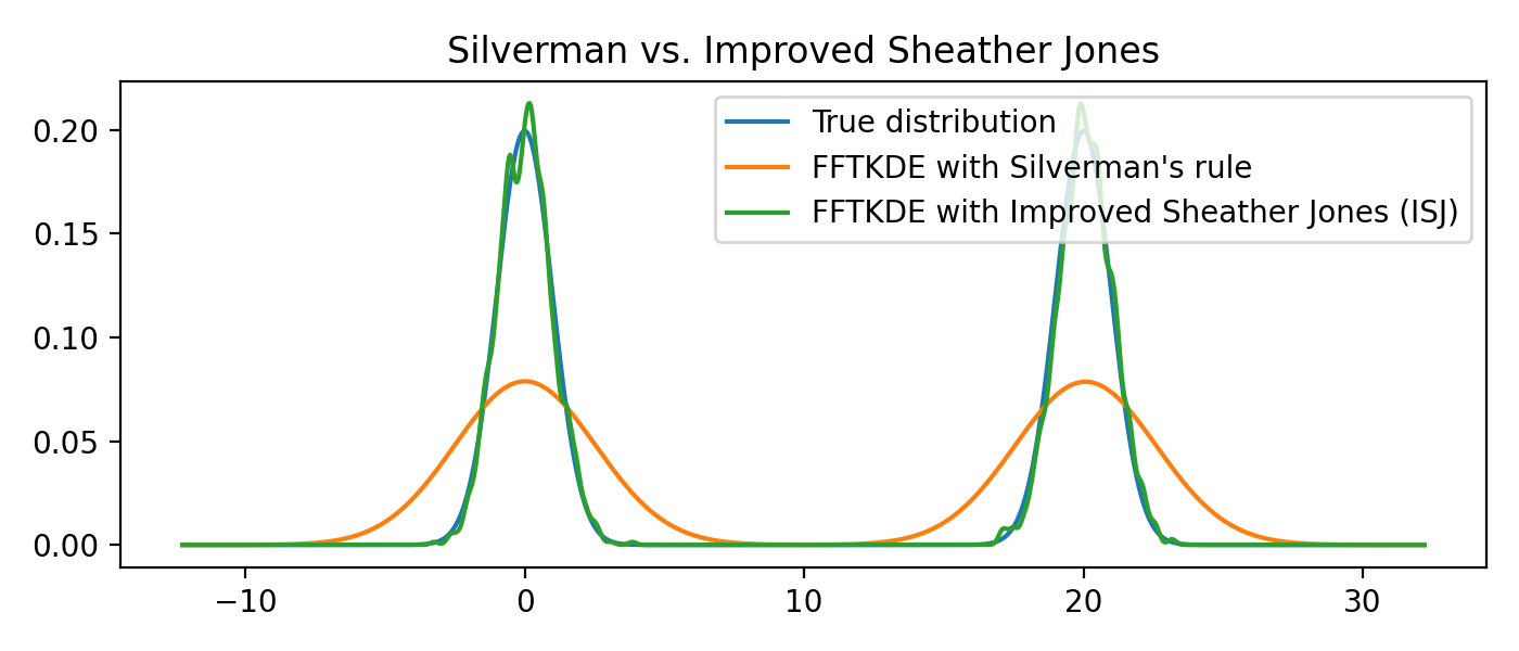
Multimodal distributions

The Improved Sheather Jones (ISJ) algorithm for automatic bandwidth selection is implemented in KDEpy. It does not assume normality, and is robust to multimodal distributions. The disadvantage is that it requires more data to make accurate assessments, and that the running time is slower.

from scipy import stats
from KDEpy import FFTKDE

# Create a bimodal distribution from two Gaussians and draw data
dist1 = stats.norm(loc=0, scale=1)
dist2 = stats.norm(loc=20, scale=1)
data = np.hstack([dist1.rvs(10**3), dist2.rvs(10**3)])

# Plot the true distribution and KDE using Silverman's Rule
x, y = FFTKDE(bw='silverman').fit(data)()
plt.plot(x, (dist1.pdf(x) + dist2.pdf(x)) / 2, label='True distribution')
plt.plot(x, y, label="FFTKDE with Silverman's rule")

# KDE using ISJ - robust to multimodality, but needs more data
y = FFTKDE(bw='ISJ').fit(data)(x)
plt.plot(x, y, label="FFTKDE with Improved Sheather Jones (ISJ)")

plt.title('Silverman vs. Improved Sheather Jones')
plt.tight_layout(); plt.legend(loc='best');

(Source code, png, hires.png, pdf)

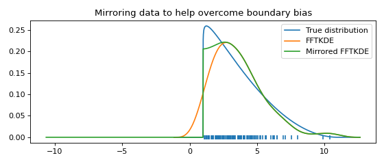
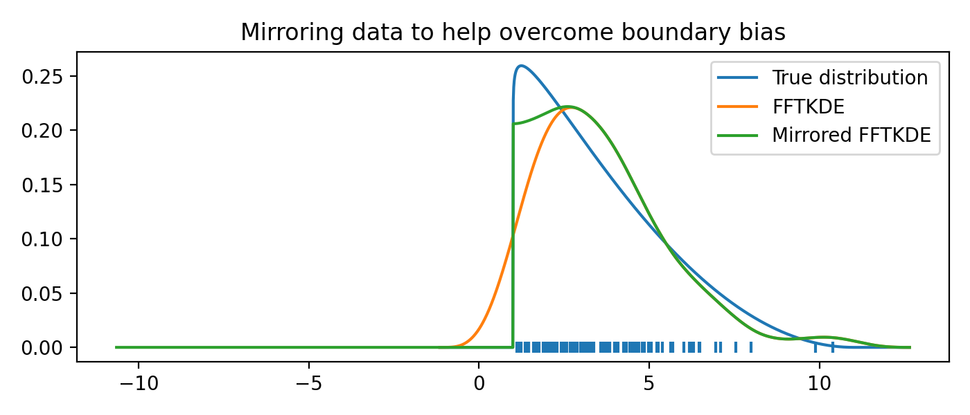
Boundary correction using mirroring

If the domain is bounded (e.g. \(\mathbb{R}_+\)) and you expect observations to fall near the boundary, a KDE might put density outside of the domain. Mirroring the data about the boundary is an elementary way to reduce this unfortunate effect. If \(\hat{g}(x)\) is the original KDE, then \(\hat{g}_*(x)=\hat{g}(2a-x)\) is the KDE obtained when mirroring the data about \(x=a\). Note that at the boundary \(a\), the derivative of the final estimate \(\hat{f}(x)\) is zero, since

\[\hat{f}'(a) = \hat{g}'(x) + \hat{g}_*'(x) \bigr |_a = \hat{g}'(x) - \hat{g}'(2a - x) \bigr |_a = \hat{g}'(a) - \hat{g}'(a) = 0,\]

where the change of sign is due to the chain rule of calculus. The reduction of boundary bias and the fact that the derivative is zero is demonstrated graphically in the example below.

from scipy import stats
from KDEpy import FFTKDE

# Beta distribution, where x=1 is a hard lower limit
dist = stats.beta(a=1.05, b=3, loc=1, scale=10)

data = dist.rvs(10**2)
kde = FFTKDE(bw='silverman', kernel='triweight')
x, y = kde.fit(data)(2**10)  # Two-step proceudure to get bw
plt.plot(x, dist.pdf(x), label='True distribution')
plt.plot(x, y, label='FFTKDE')
plt.scatter(data, np.zeros_like(data), marker='|')

# Mirror the data about the domain boundary
low_bound = 1
data = np.concatenate((data, 2 * low_bound - data))

# Compute KDE using the bandwidth found, and twice as many grid points
x, y = FFTKDE(bw=kde.bw, kernel='triweight').fit(data)(2**11)
y[x<=low_bound] = 0  # Set the KDE to zero outside of the domain
y = y * 2  # Double the y-values to get integral of ~1

plt.plot(x, y, label='Mirrored FFTKDE')
plt.title('Mirroring data to help overcome boundary bias')
plt.tight_layout(); plt.legend();

(Source code, png, hires.png, pdf)

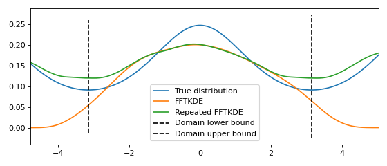
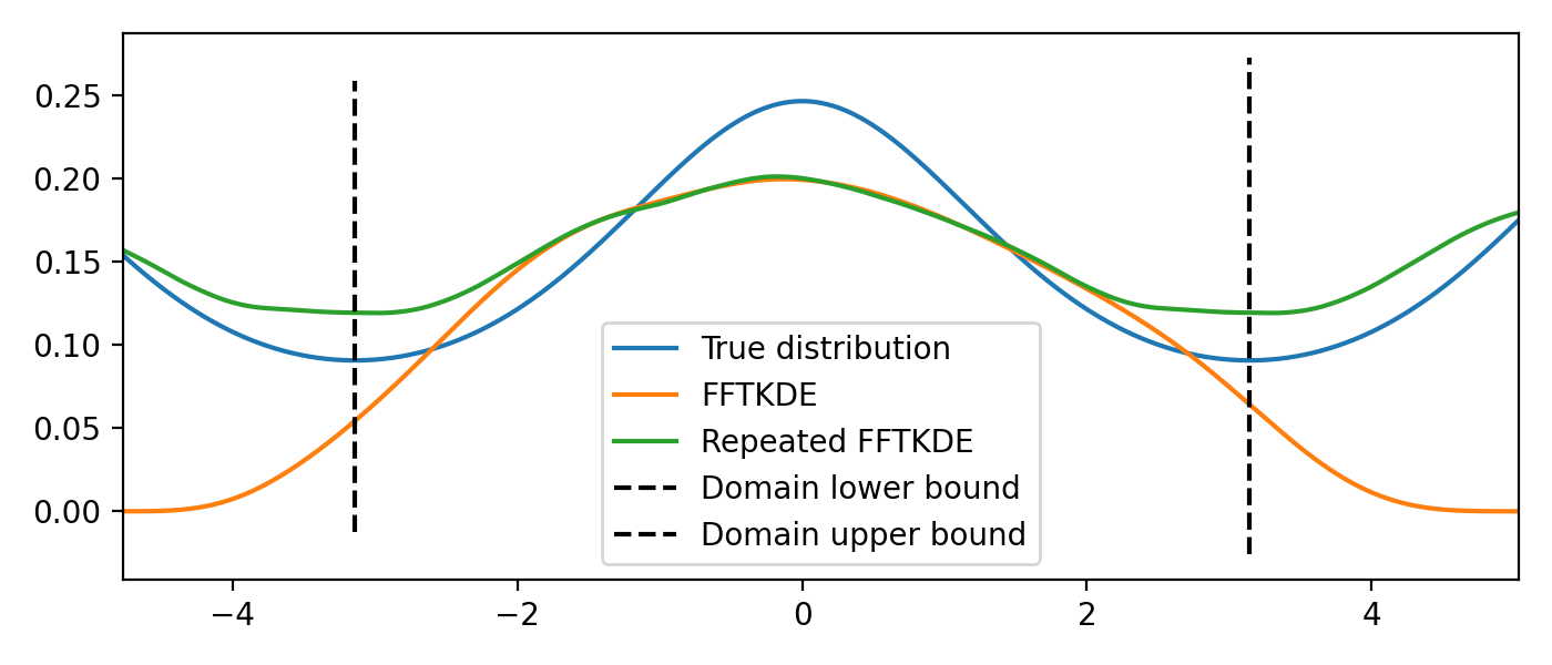
Estimating density on the circle

If the data is bounded on a circle and the domain is known, the data can be repeated instead of reflected. The result of this is shown graphically below. The derivative of \(\hat{f}(x)\) at the lower and upper boundary will have the same value.

from scipy import stats
from KDEpy import FFTKDE

# The Von Mises distribution - normal distribution on a circle
dist = stats.vonmises(kappa=0.5)
data = dist.rvs(10**2)

# Plot the normal KDE and the true density
kde = FFTKDE(bw='silverman', kernel='triweight')
x, y = kde.fit(data).evaluate()
plt.plot(x, dist.pdf(x), label='True distribution')
plt.plot(x, y, label='FFTKDE')
plt.xlim([np.min(x), np.max(x)])

# Repeat the data and fit a KDE to adjust for boundary effects
a, b = (-np.pi, np.pi)
data = np.concatenate((data - (b - a), data, data + (b - a)))
x, y = FFTKDE(bw=kde.bw, kernel='biweight').fit(data).evaluate()
y = y * 3  # Multiply by three since we tripled data observations

plt.plot(x, y, label='Repeated FFTKDE')
plt.plot([a, a], list(plt.ylim()), '--k', label='Domain lower bound')
plt.plot([b, b], list(plt.ylim()), '--k', label='Domain upper bound')
plt.tight_layout(); plt.legend();

(Source code, png, hires.png, pdf)

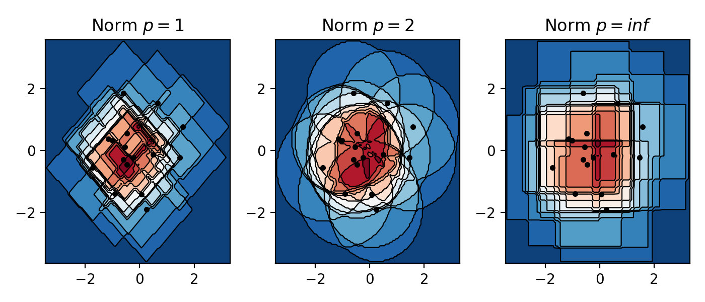
The effect of norms in 2D

Below a non-smooth kernel is chosen to reveal the effect of the choice of norm more clearly.

from KDEpy import FFTKDE

# Create 2D data of shape (obs, dims)
data = np.random.randn(2**4, 2)

grid_points = 2**7  # Grid points in each dimension
N = 16  # Number of contours

for plt_num, norm in enumerate([1, 2, np.inf], 1):

    ax = fig.add_subplot(1, 3, plt_num)
    ax.set_title(f'Norm $p={norm}$')

    # Compute the kernel density estimate
    kde = FFTKDE(kernel='box', norm=norm)
    grid, points = kde.fit(data).evaluate(grid_points)

    # The grid is of shape (obs, dims), points are of shape (obs, 1)
    x, y = np.unique(grid[:, 0]), np.unique(grid[:, 1])
    z = points.reshape(grid_points, grid_points).T

    # Plot the kernel density estimate
    ax.contour(x, y, z, N, linewidths=0.8, colors='k')
    ax.contourf(x, y, z, N, cmap="RdBu_r")
    ax.plot(data[:, 0], data[:, 1], 'ok', ms=3)

plt.tight_layout()

(Source code, png, hires.png, pdf)

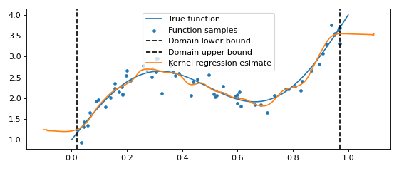
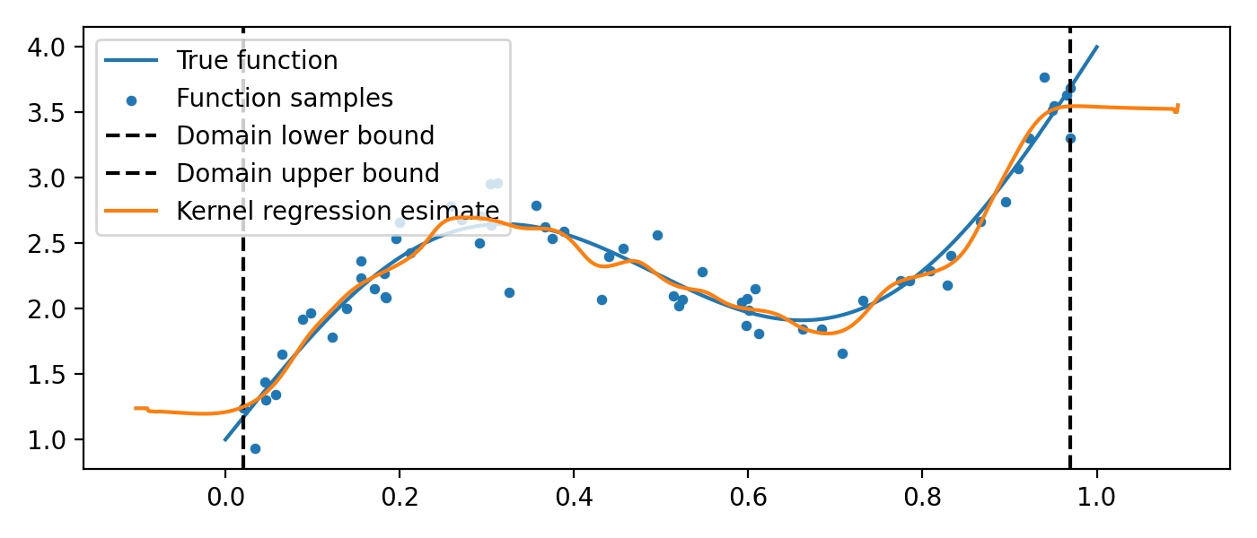
One dimensional kernel regression

One dimensional kernel regression seeks to find \(\hat{y} = \mathbb{E}[y | x]\). This can be elegantly computed by first modeling the full distribution \(p(x, y)\). We have that

\[\hat{y} = \mathbb{E}[y | x] = \int p(y | x) y \, dy = \sum_i p(y_i | x) y_i = \sum_i \frac{p(y_i, x)}{\sum_j p(y_j, x)} y_i\]

Modelling the distribution \(p(y | x)\) only to infer \(\mathbb{E}[y | x]\) is generally wasteful, but the speed of the FFTKDE implementation makes the approach tractable. A million points should pose no problem. Extensions to model the conditional variance \(\operatorname{var}[y | x]\) are possible too.

from KDEpy import FFTKDE
func = lambda x : np.sin(x * 2 * np.pi) + (x + 1)**2

# Generate random data
num_data_points = 2**6
data_x = np.sort(np.random.rand(num_data_points))
data_y = func(data_x) + np.random.randn(num_data_points) / 5

# Plot the true function and the sampled values
x_smooth = np.linspace(0, 1, num=2**10)
plt.plot(x_smooth, func(x_smooth), label='True function')
plt.scatter(data_x, data_y, label='Function samples', s=10)

# Grid points in the x and y direction
grid_points_x, grid_points_y = 2**10, 2**4

# Stack the data for 2D input, compute the KDE
data = np.vstack((data_x, data_y)).T
kde = FFTKDE(bw=0.025).fit(data)
grid, points = kde.evaluate((grid_points_x, grid_points_y))

# Retrieve grid values, reshape output and plot boundaries
x, y = np.unique(grid[:, 0]), np.unique(grid[:, 1])
z = points.reshape(grid_points_x, grid_points_y)
plt.axvline(np.min(data_x), ls='--', c='k', label='Domain lower bound')
plt.axvline(np.max(data_x), ls='--', c='k', label='Domain upper bound')

# Compute y_pred = E[y | x] = sum_y p(y | x) * y
y_pred =  np.sum((z.T / np.sum(z, axis=1)).T  * y , axis=1)
plt.plot(x, y_pred, zorder=25, label='Kernel regression esimate')

plt.legend(); plt.tight_layout()

(Source code, png, hires.png, pdf)

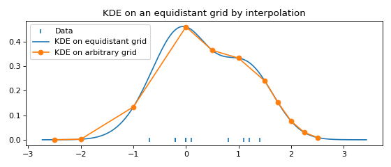
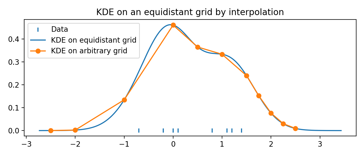
Fast evaluation on a non-equidistant grid

For plotting and in most computations, an equidistant grid is exactly what we want. To evaluate the FFTKDE on an arbitrary grid, we can make use of scipy.

from KDEpy import FFTKDE
from scipy.interpolate import interp1d

data = [-0.7, -0.2, -0.2, -0.0, 0.0, 0.1, 0.8, 1.1, 1.2, 1.4]
x, y = FFTKDE(bw="silverman").fit(data).evaluate()

# Use scipy to interplate and evaluate on arbitrary grid
x_grid = np.array([-2.5, -2, -1, 0, 0.5, 1, 1.5, 1.75, 2, 2.25, 2.5])
f = interp1d(x, y, kind="linear", assume_sorted=True)
y_grid = f(x_grid)

# Plot the resulting KDEs
plt.scatter(data, np.zeros_like(data), marker='|', label="Data")
plt.plot(x, y, label="KDE on equidistant grid")
plt.plot(x_grid, y_grid, '-o', label="KDE on arbitrary grid")
plt.title('KDE on an equidistant grid by interpolation')
plt.tight_layout(); plt.legend(loc='upper left');

(Source code, png, hires.png, pdf)