Kernels
Available kernels
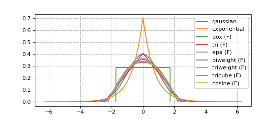
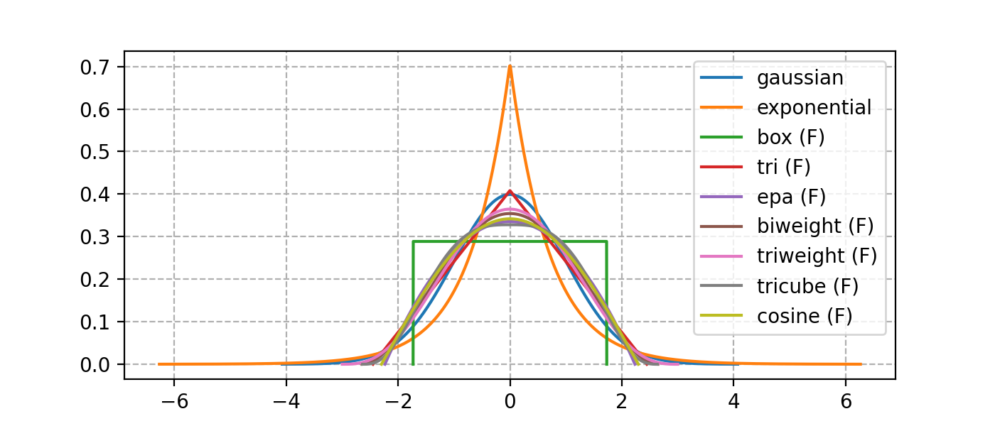
You are likely reading this because you wonder which kernel functions \(K\) are available.
Every available kernel is shown in the figure below.
Kernels with finite support (synonymous with bounded support in these docs) are annotated with an F.
A listing of every available option is found in NaiveKDE._available_kernels.keys().
from KDEpy import NaiveKDE

for name, func in NaiveKDE._available_kernels.items():
   x, y = NaiveKDE(kernel=name).fit([0]).evaluate()
   plt.plot(x, y, label=name + (' (F)' if func.finite_support else ''))

plt.grid(True, ls='--', zorder=-15); plt.legend();
(Source code, png, hires.png, pdf)
Kernel properties
The kernels implemented in KDEpy obey some common properties.
Normalization: \(\int K(x) \, dx = 1\).
Unit variance: \(\operatorname{Var}[K(x)] = 1\) when the bandwidth \(h\) is 1. The bandwith of the each kernel equals its standard deviation.
Symmetry: \(K(-x) = K(x)\) for every \(x\).
Kernels are radial basis functions
Symmetry follows from a more general property, namely the fact that every kernel implemented is a radial basis function. A radial basis function is a function which evaluates to the same value whenever the distance from the origin is the same. In other words, it is the composition of a norm \(\left\| \cdot \right\| _p: \mathbb{R}^d \to \mathbb{R}_+\) and a function \(\kappa: \mathbb{R}_+ \to \mathbb{R}_+\).
Note
If you have high dimensional data with different scales, consider standardizing the data before feeding it to a KDE.
Kernels may have finite support, or not
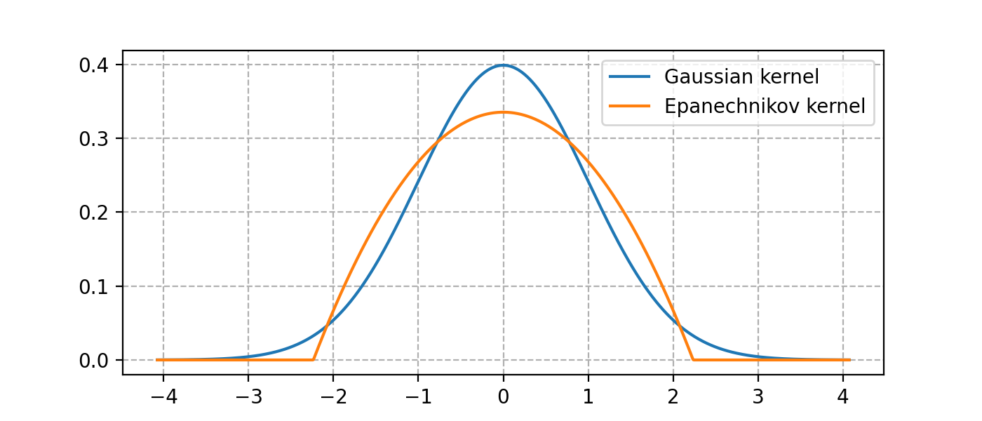
A given kernel may or may not have finite support. A kernel with finite (or bounded) support is defined on a domain such as \([-1, 1]\), while a kernel without finite support is defined on \((-\infty, \infty)\).
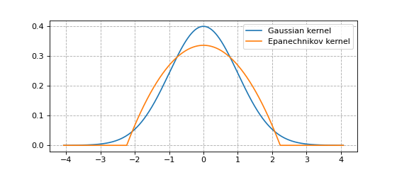
Below we plot the Guassian kernel and the Epanechnikov kernel.
The Gaussian kernel does not have finite support.
The Epanechnikov kernel has finite support.
The reason why kernels are normalized to unit variance is so that bounded and non-bounded
kernel functions are more easily compared.
In other words, setting bw=1 in the software ensures that the standard deviation \(\sigma = 1\).
from KDEpy import *

x, y1 = NaiveKDE(kernel='gaussian', bw=1).fit([0]).evaluate()
y2 = NaiveKDE(kernel='epa', bw=1).fit([0]).evaluate(x)
plt.plot(x, y1, label='Gaussian kernel')
plt.plot(x, y2, label='Epanechnikov kernel')
plt.grid(True, ls='--', zorder=-15); plt.legend();
(Source code, png, hires.png, pdf)
Higher dimensional kernels
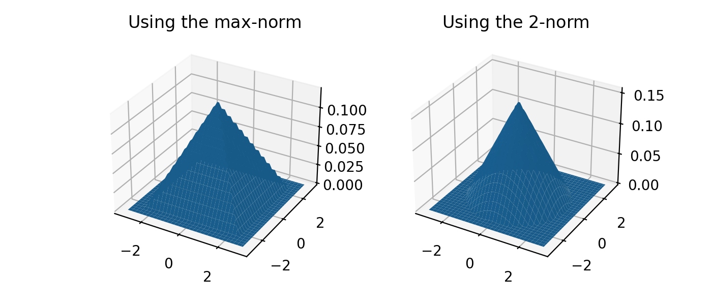
The one-dimensional example is deceptively simple, since in one dimension every \(p\)-norm is equivalent. In higher dimensions, this is not true. The general \(p\)-norm is a measure of distance in \(\mathbb{R}^d\), defined by
The three most common \(p\)-norms are
The Manhattan norm \(\left\| x \right\| _1 = \sum_{i} \left| x_i \right|\)
The Euclidean norm \(\left\| x \right\| _2 = \sqrt{x_1^2 + x_2^2 + \dots + x_d^2}\)
The max-norm \(\left\| x \right\| _\infty = \max_{i} \left| x_i \right|\)
In higher dimensions, a norm must be chosen in addition to a kernel. Let \(r := \left\| x \right\| _p\) be a measure of distance (\(r\) stands for radius here). The normalization necessary to ensure \(\int \kappa ( \left\| x \right\| _p ) \, dx = 1\) depends on the value of \(p\), but symmetry is guaranteed since \(\left\| -x \right\| _p = \left\| x \right\| _p\). The figure below shows the effect of choosing different norms with the same kernel.
from KDEpy.BaseKDE import BaseKDE
from mpl_toolkits.mplot3d import Axes3D

kernel = BaseKDE._available_kernels['tri']

n = 64
p = np.linspace(-3, 3, num=n)
obs_x_dims = np.array(np.meshgrid(p, p)).T.reshape(-1, 2)

ax = fig.add_subplot(1, 2, 1, projection='3d')
z = kernel(obs_x_dims, norm=np.inf).reshape((n, n))
surf = ax.plot_surface(*np.meshgrid(p, p), z)
ax.set_title('Using the $\max$-norm')

ax = fig.add_subplot(1, 2, 2, projection='3d')
z = kernel(obs_x_dims, norm=2).reshape((n, n))
surf = ax.plot_surface(*np.meshgrid(p, p), z)
ax.set_title('Using the $2$-norm')
(Source code, png, hires.png, pdf)

Kernel normalization
Kernels in any dimension are normalized so that the integral is unity for any \(p\). To explain how a high-dimensional kernel is normalized, we first examine high dimensional volumes.
Let \(r := \left\| x \right\| _p\) be the distance from the origin, as measured by some \(p\)-norm. The \(d\)-dimensional volume \(V_d(r)\) is proportional to \(r^d\). We will now examine the unit \(d\)-dimensional volume \(V_d := V_d(1)\).
We integrate over a \(d-1\) dimensional surface \(S_{d-1}(r)\) to obtain \(V_{d}\) using
Since a \(d-1\) dimensional surface is proportional to \(r^{d-1}\), we write it as \(S_{d-1}(r) = K_{d-1} r^{d-1}\), where \(K_{d-1}\) is a constant. Pulling this out of the integral, we are left with
From this we observe that \(K_{d-1} = V_d \cdot d\), a fact we’ll use later.
What is the volume of a unit ball \(V_d\) in the \(p\) norm in \(d\) dimensions? Fortunately an analytical expression exists, it’s given by
For more information about this, see for instance the paper by Wang in Literature review, where we have used \(K_{d-1} = V_d \cdot d\). The equation above reduces to more well-known cases when \(p\) takes common values, as shown in the table below.
\(p\) |
Name |
Unit volume \(V_d\) |
|---|---|---|
\(1\) |
Cross-polytope |
\(\frac{2^d}{d!}\) |
\(2\) |
Hypersphere |
\(\frac{\pi^{d/2}}{\Gamma\left ( \frac{d}{2} + 1 \right )}\) |
\(\infty\) |
Hypercube |
\(2^d\) |
Example - normalization
We would like to normalize kernel functions in higher dimensions for any norm. To accomplish this, we start with the equation for the volume of a \(d\)-dimensional volume. The equation is
The integral of the kernel \(\kappa: \mathbb{R}_+ \to \mathbb{R}_+\) over the \(d\)-dimensional space is then given by
which we can compute. For instance, the linear kernel \(\kappa(r) = (1-r)\) is normalized by
The biweight kernel \(\kappa(r) = \left ( 1 - r^2 \right )^2\) is similarly normalized by
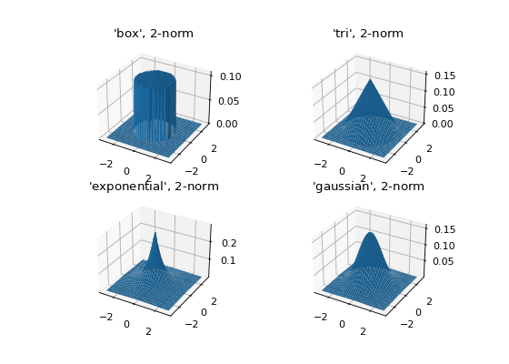
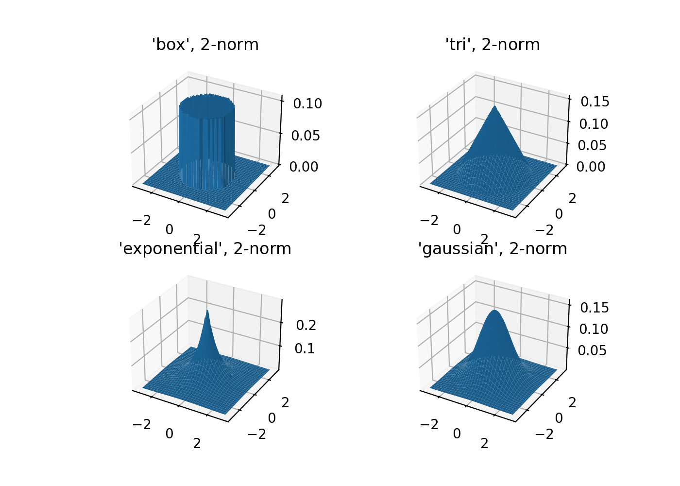
Some 2D kernels
Let’s see what the kernels look like in 2D when \(p=2\).
from KDEpy.BaseKDE import BaseKDE
from mpl_toolkits.mplot3d import Axes3D

n = 64
p = np.linspace(-3, 3, num=n)
obs_x_dims = np.array(np.meshgrid(p, p)).T.reshape(-1, 2)

# fig = plt.figure() is already set, adjust the size
fig.set_figwidth(7); fig.set_figheight(5);

selected_kernels = ['box', 'tri', 'exponential', 'gaussian']
for i, kernel_name in enumerate(selected_kernels, 1):

  kernel = BaseKDE._available_kernels[kernel_name]
  ax = fig.add_subplot(2, 2, i, projection='3d')
  z = kernel(obs_x_dims, norm=2).reshape((n, n))
  surf = ax.plot_surface(*np.meshgrid(p, p), z)
  ax.set_title(f"'{kernel_name}', $2$-norm")
(Source code, png, hires.png, pdf)
